This series includes the Machine Learning course notes which I collected while I was in the course phase at Ph.D.
Training Approaches
Machine Learning training approaches divide into 3;
- Supervised Learning
- Unsupervised Learning
- Reinforcement Learning
ID3 Decision Tree
- This approach is known as supervised and non-parametric decision tree type.
- Mostly, it is used for classification and regression.
- A tree consists of an inter decision node and terminal leaves. And terminal leaves have outputs. The output display class values in classification, however, display numeric value for regression.
- The aim of dividing subsets into decision trees is to make each subset as homogeneous as possible. The disadvantage of decision tree algorithms is that they are greedy approaches. A Greedy algorithm is any algorithm that follows the problem solving heuristic of making the locally optimal choice at each stage with the intent of finding a global optimum. In many problems, a greedy strategy does not usually produce an optimal solution, but nonetheless a greedy heuristic may yield locally optimal solutions that approximate a globally optimal solution in a reasonable amount of time.

Entropy
Entropy known as the controller for decision tree to decide where to split the data. ID3 algorithm uses entropy to calculate the homogeneity of a sample. If the sample is completely homogeneous the entropy is zero and if the sample is an equally divided it has entropy of one[1].
n-class Entropy -> E(S) = ∑ -(pᵢ*log₂pᵢ)
2-class Entropy: (S) =-(p₁ * log₂p₁ + p₂ * log₂p₂)
Ex-1:

p₁ = 9/(9+5) =9/14 (probability of a sample in the same training class with class 1)
p₂ = 5/14 (probability of a sample in the same training class with class 2)
E = -(9/14 * log₂(9/14) + (5/14) * log₂(5/14))
E = 0.94
Information Gain
The boundaries of root, nodes and leaves are defined by Information Gain (IG).
Gain(S,A) = E(before) – G(after_splitting)
Note: You can find ID3 as C4.5 in WEKA Tool.
Ex 2:

First, select the feature that will divide the whole table in the most accurate way. For this, the feature that gives the highest gain should be determined.
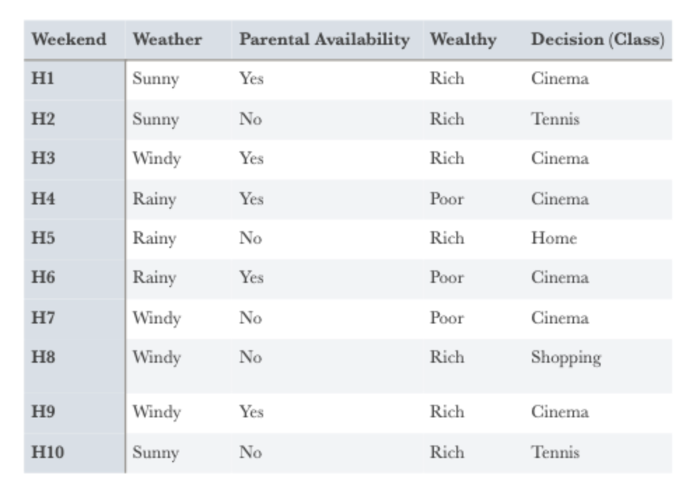
Values for 10 training examples are divided as follows:
* 6 Cinema
* 2 Tennis
* 1 House
* 1 Shopping
Entropy value must be calculated from these values for the beginning to define root feature.
E(S) = -((6/10)*log2(6/10) + (2/10)*log2(2/10) + (1/10)*log2(1/10) + (1/10)*log2(1/10))
E(S) = 1.571
By calculating the gain values of all individual features, the features with the highest gain value is selected as the root node:
Gain(S,Weather) = ?
Sunny = 3 (1 Cinema + 2 Tennis)
Windy = 4 (3 Cinema + 1 Shopping)
Rainy = 3 (2 Cinema + 1 Home)
Entropy(Ssunny)= — (1/3)*log2(1/3) — (2/3)*log2(2/3) = 0.918
Entropy(Swindy)= — (3/4)*log2(3/4) — (1/4)*log2(1/4) = 0.811
Entropy(Srainy)= — (2/3)*log2(2/3) — (1/3)*log2(1/3) = 0.918

Gain(S, Weather) = 1.571 — (((1+2)/10)*0.918 + ((3+1)/10)*0.811 + ((2+1)/10)*0.918)
Gain(S, Weather) = 0.70
Gain(S, Parental_Availability) = ?
Yes = 5 (5 Cinema)
No = 5 (2 Tennis + 1 Cinema + 1 Shopping + 1 Home)
Entropy(Syes) = – (5/5)*log2(5/5) = 0
Entropy(Sno) = -(2/5)*log2(2/5) -3*(1/5)*log2(1/5) = 1.922
Gain(S, Parental_Availability) = Entropy(S) — (P(yes)*Entropy(Syes) + P(no)*Entropy(Sno))
Gain(S, Parental_Availability) = 1.571 — ((5/10)*Entropy(Syes) + (5/10)*Entropy(Sno))
Gain(S, Parental_Availability) = 0.61
Gain(S, Wealth)=?
Rich = 7 (3 Cinema + 2 Tennis + 1 Shopping + 1 Home)
Poor = 3 (3 Sinema)
Entropy(Srich) = 1.842
Entropy(Spoor)=0
Gain(S, Wealth) = Entropy(S) — (P(rich)*Entropy(Srich) + P(poor)*Entropy(Spoor))
Gain(S, Wealth) = 0.2816
Finally, all gain values are listed one by one and the feature with the highest gain value is selected as the root node. In this case weather has the highest gain value so It will be the root.
Gain(S, Weather) = 0.70
Gain(S, Parental_Availability) = 0.61
Gain(S, Wealth) = 0.2816

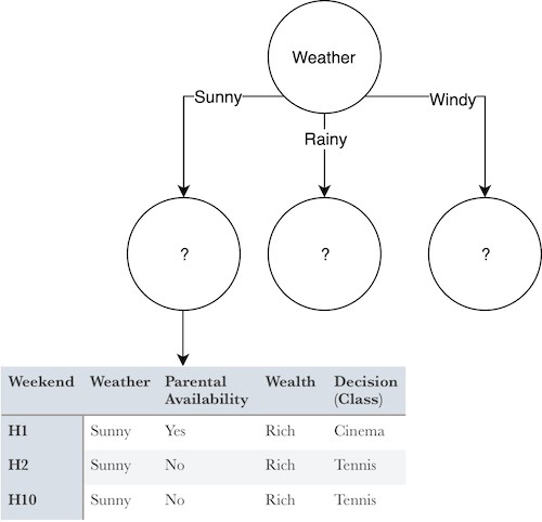
As shown in the above example, after selecting the root, each of the individual values of the features are determined as leaves and this time the data set is customized with these individual values. In other words, the table above has been converted to a separate data set showing the values that other features can take if the weather is Sunny. Thus, when the weather is sunny, according to this table, the possible classes of the inter node will be as follow:
- 1 Cinema
- 2 Tennis
Entropy(Ssunny) = -(1/3)*log2(1/3) -(2/3)*log2(2/3) = 0.918
Gain(Ssunny,Parental_Availability) = ?
Gain(Ssunny,Parental_Availability) = Entropy(Ssunny) — (P(yes |Ssunny)*Entropy(Syes) + P(no |Ssunny)*Entropy(Sno))
Entropy(Syes) = -(1/3)*log2(0) — 0 = 0
Entropy(Sno) = -(2/3)*log2(0) — 0 = 0
Gain(Ssunny,Parental_Availability)= 0.928 — ((1/3)*0 + (2/3)*0) = 0.928
Gain(Ssunny, Wealth) = 0.918 — ((3/3)*0.918 + (0/3)*0) = 0
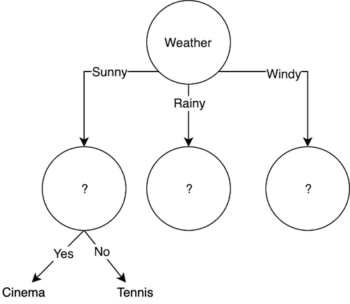
Because the gain of the Parental_Availability feature is greater, the leaf of the Sunny state will be Parental_Availability. According to the data set for sunny conditions, if yes, Cinema will be decided and if no, then Tennis will be decided:

When the same calculations are made for Windy and Rainy situations, the final decision tree will be completed.
Overfitting
- It is the transformation of learning into memorization.
- The performance graph is that after a certain moment, the increase in performance stops and starts to decrease.
- When your success rate high for training performance but opposite for test performance is an example for overfitting.
- Moreover, if there is a noisy sample in our data, it may cause overfitting.
- When the tree grows too large, a result is produced for almost every possible branch, which leads to overfitting.
In order to avoid overfitting, it is necessary to prun the tree either when it is growing or after the tree is formed.
References:
[1] Decision Tree, https://www.saedsayad.com/decision_tree.htm